Neural Kalman Filters for
Acoustic Echo Cancellation

Ernst Seidel, Gerald Enzner, Pejman Mowlaee, Tim Fingscheidt (2024)

汇报人:SZ2503007 丁阳奕
演讲时间:2026.4.20
Paper Page 3 Paper Page 2 Paper Page 1

1. The Acoustic Echo Problem

Hands-free & Speakerphone Scenarios

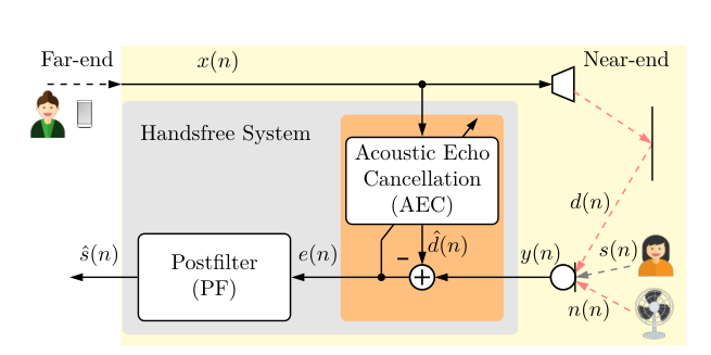
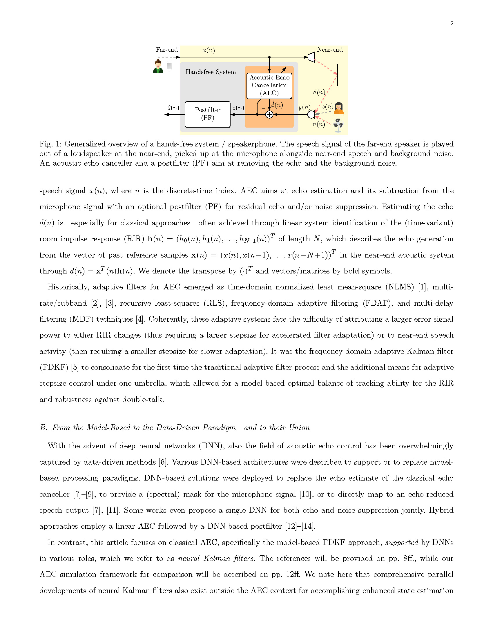
  • The Loop: Far-end speech x(n) plays through a loudspeaker, travels through the room, and is picked up by the microphone as echo.
  • Signal Mixture: The mic signal y(n) = s(n) + n(n) + d(n), where s(n) is Near-end speech, n(n) is Background noise, and d(n) is Echo.
  • The Goal: Use the reference x(n) to estimate and subtract the echo.
  • The Challenge: It's not just about "lowering volume". During double-talk, the algorithm must suppress echo but preserve near-end speech, and adapt quickly when the echo path changes.
AEC System Overview
Fig 1: Signal relationships in an AEC system

2. From Adaptive Filtering to Frequency-Domain Kalman Filter(FDKF)

State-Space Modeling for AEC

Linear Echo Model

d(n) = xT(n)h(n)

The Real Difficulty

A large error may mean either echo-path change or near-end/noise interference

Step-Size Dilemma

Large μ: fast adaptation but harms near-end speech
Small μ: safer but slow reconvergence

LMS / NLMS

d(n) = xT(n)h(n)
e(n) = y(n) - xT(n)ĥ(n-1)
ĥ(n) = ĥ(n-1) + μ e(n)x(n)
μ = μ0 / ‖x(n)‖2 for NLMS
  • update strength is controlled by μ
  • but e(n) mixes path mismatch and near-end/noise interference
  • therefore a single heuristic step size cannot balance fast tracking and double-talk robustness
LMS/NLMS updates the filter, but does not model why the error became large.

FDKF

State model:
h(n+1) = ah(n) + Δh(n)
Kalman update:
+(n) = ĥ(n-1) + k(n)e(n)
Kalman gain:
k(n) = p(n)x(n)(xT(n)p(n)x(n) + σ2s+n(n))-1
  • large p(n) means the model is uncertain, so adapt more
  • large σ2s+n(n) means the observation is noisy, so adapt less
  • therefore Kalman gain acts as a model-based adaptive step size

Why frequency-domain?

  • decorrelates near-end speech/noise approximately
  • reduces computational complexity
  • enables practical per-bin Kalman adaptation
FDKF models both path variation and observation noise in one framework.

3. Why Neural Kalman Filters?

Combining the Best of Both Worlds

Neural Kalman Overview
Fig 2: Neural Kalman / FDKF Framework (Right: injectable DNN modules)
  • FDKF Advantages: Low complexity, few parameters, clear structure, excellent near-end speech protection.
  • FDKF Weaknesses: Strong linear assumptions (fails on loudspeaker nonlinearities), hard to estimate covariance priors accurately.
  • Pure DNN AEC: Powerful, but often requires massive models or sacrifices near-end speech quality (aggressive suppression).
  • The Hybrid Approach: Keep the FDKF state-space skeleton, but let the DNN learn the hardest-to-model local components:
    • Distortion Model — handle loudspeaker nonlinearity
    • Filter-State Update — refine the state recursion
    • Kalman Gain — improve adaptation control

4. Where Exactly Does the DNN Go?

Architectural Variations

Architectures
Fig 3: Internal structures of NeuralKalman vs DeepAdaptive
Method What the DNN Learns Architecture Type Characteristics
FDKF (None - fully statistical) N/A Baseline, lowest complexity
DLAC-Kalman / NKF Kalman Gain (State Uncertainty) Per-Bin (Shared small network) High flexibility, fewer params, but higher FLOPS
NeuralKalman Distortion + Dynamic State Update Fully Connected (Joint-Freq) Balanced, lower FLOPS, Kalman gain stays model-based
DeepAdaptive Distortion + DNN-based Kalman Gain Fully Connected (Joint-Freq) Acts more like an aggressive suppressor, higher risk to near-end

5. Fair Experimental Setup

Ensuring an Apples-to-Apples Comparison

  • Unified Framework: All compared methods are implemented in one common framework; all hybrid models are trained from scratch in PyTorch.
  • Strict Constraints: 16 kHz sampling rate, matched algorithmic delay, and aligned effective reference input length.
  • Evaluation Datasets (Unseen Data):
    • Dtest: Standard speech far-end excitation.
    • DWGN_test: White Gaussian Noise far-end.
    • DNL_test: Strong loudspeaker non-linearities.
  • Segments include Single-Talk Far-End (STFE), Near-End (STNE), and Double-Talk (DT).
Training
VCTK + Synthetic RIR + SEF NL + DEMAND/QUT Noise
PyTorch Unified AEC Framework
Testing
TIMIT + Real Aachen RIR + ETSI Noise
Metrics: ERLE, AECMOS, PESQ, STOI, LPS, FLOPS, Params

6. Convergence Behavior (Single Example)

ERLE over time in Dtest

  • Initial STFE Phase: All neural Kalman filters reach higher Echo Return Loss Enhancement (ERLE) much faster than the standard FDKF.
  • DeepAdaptive: most aggressive echo reduction, consistent with suppressor-like behavior.
  • NKF & DLAC-Kalman: more balanced across STFE and DT
  • NeuralKalman: lower ERLE overall, but less drop during low-power far-end segments
  • Double-Talk (DT): Overall ERLE naturally drops. Reminder: high suppression during DT often correlates with near-end speech degradation
Dtest single example
Fig 4: Time-domain signals and ERLE curves across STFE, STNE, and DT segments.

7. Re-convergence After RIR Switch

Adapting to Sudden Echo Path Changes (at 4s)

  • FDKF Shortcoming: Updates are too conservative, leading to painfully slow re-convergence (Fig 5).
  • Speech Excitation: DeepAdaptive reconverges the fastest; NeuralKalman also recovers rapidly. NKF and DLAC-Kalman are steadier but still clearly outperform FDKF.
  • WGN Excitation (Stress Test): NKF, DLAC-Kalman, and FDKF reach solid final accuracy, while DeepAdaptive and NeuralKalman are limited to about 10 dB ERLE.
  • However, DeepAdaptive & NeuralKalman struggle under WGN excitation, suggesting that fast reconvergence in speech conditions may partly come from masking behavior rather than true echo-path tracking.
Speech Re-convergence WGN Re-convergence
Fig 5 (Top): Speech Excitation. Fig 6 (Bottom): WGN Excitation.

8. Suppression vs. Preservation

Comprehensive Double-Talk Performance

  • Echo Suppression: DeepAdaptive leads in ERLE/AECMOS Echo, acting as a strong suppressor.
  • Near-End Preservation: DLAC-Kalman leads neural models in PESQ, STOI, and LPS. Learning the Kalman gain appears to be the most balanced way to improve FDKF while preserving near-end speech.
  • The Trade-off: DeepAdaptive shows the strongest suppression but pays a clearer price in speech quality; NeuralKalman shows a similar tendency.
  • Non-linearities (Red lines): DNL_test severely impacts speech quality metrics, even if ERLE looks okay.
  • Resources: FDKF is cheapest. NKF/DLAC have few parameters but high FLOPS. Fully connected hybrids have low FLOPS but high parameters.
Comprehensive Metrics
Fig 7: Echo metrics, Speech metrics, and Complexity (Blue = Linear, Red = Non-linear)

9. Conclusions & Design Implications

What this paper suggests for next-generation AEC

1. Hybrid beats standard FDKF

  • Faster convergence
  • Stronger echo suppression
  • Better overall adaptation

2. Gain-focused learning is the most balanced

  • Better near-end speech preservation
  • Strong performance without over-aggressive suppression
  • Best represented by DLAC-Kalman / NKF

3. Architecture still matters

  • Per-bin (NKF / DLAC-Kalman): flexible, parameter-light, high FLOPS
  • Fully connected: lower FLOPS, more parameters, less flexibility
  • Postfilter: still necessary for nonlinear and long-tail residual echo

Thank You

×

1 / 11